
more neurocat Workshops can be found in the official blog
Prioritized Experience Replay
Review and ideas for the paper Prioritized Experience Replay, by Google DeepMind.
Introduction
One reason of the great success in Reinforcement Learning (RL) was the introduction of experience replay. This smooths the training distribution uniformly over past behavior of the RL agent. Unfortunately this implies transitions get replayed regardless of their significance in the frequency of being experienced.
This paper attacks this issue by prioritizing experience and sample due to a underlying distribution. Assuming the TD-error gives a measure for how “uncertain” a transition is, our first choice for prioritizing would be according to the transitions TD-error.
For prioritized experience replay there are different approaches.
Greedy Prioritization
The oracle based approach always samples the experience with maximal TD-Error. This sounds easy in theory. However in practice this results in expensive sorting and updating of the underlying experience. To achieve this it is plausible to introduce a binary heap structure with sorting complexity of $\mathcal{O}(\log{n})$ and sampling of the maximum value with complexity $\mathcal{O}(1)$.
Binary Heap
Lets take a look at the concept of a Binary Heap. A heap makes use of a tree structure that isn’t fully sorted but satisfies the heap property such that every node is smaller then its parent
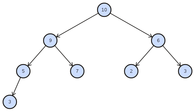
When inserting an item it gets inserted into the last position.
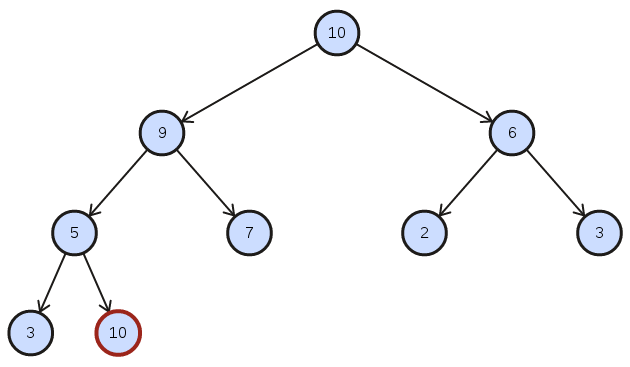
Then incrementally the heap will satisfy the heap property by percolating the item up as long as the heap property is not satisfied.
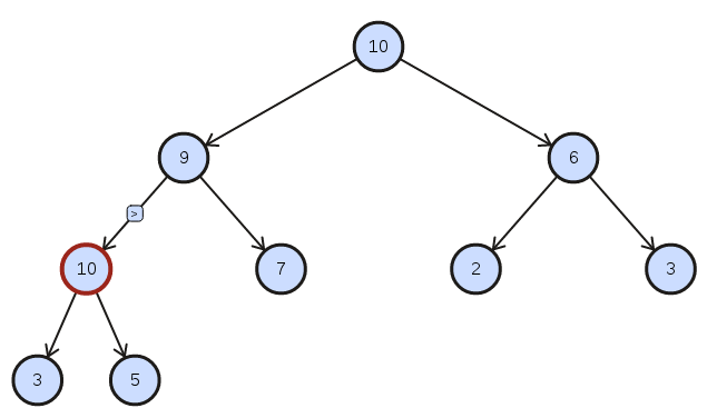
When inserting a node into a sorted heap structure the heap remains sorted after percolating up the inserted node.
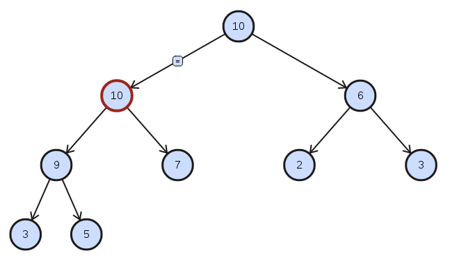
As you can see the maximal value of the heap is always the upper item. Thats why we only need $\mathcal{O}(1)$ to sample the maximal value.
Please be aware that satisfying the heap property doesn’t result in a fully sorted priority queue. When updating the value of a node it suffice to percolate (up or down) the updated node to maintain the heap property. That way we can ensure drawing the maximal value in constant time while updating the structure in $\mathcal{O}(\log{n})$.
The appendix of this post includes a manual for a concrete python inplementation of a binary heap, integrated with build-in methods to handle the heap as native as a list.
Disadvantages of Greedy Prioritization
Greedy Prioritization faces the problems that
- only replayed elements are getting updated. This means elements with small transition on the first run may never be visited.
- It is sensitive to noise spikes and
- prone to overfitting for slowly shrinking error. High initial transitions are replayed more frequently.
To overcome these issues we need to find something in the middle of uniform and greedy sampling.
Stochastic Prioritization
Stochastic Prioritization is trying to solve that problem with a monotonic probability of being drawn with guaranteeing non-zero probabilities.
For that consider a Memory with size $N$ and replay probability of element $i$ as $P(i)=\dfrac{p_{i}^{\alpha}}{\sum_{k=0}^N}p_{k}^{\alpha}$
If $\alpha=0$ we get the uniform case.
At that point we can further differentiate between stochastic prioritization approaches. Namely the proportional and the rank-based approach.
Proportional Stochastic Prioritization
We will sample experience proportional to its TD-error $\delta_{i}$. With that we satisfy a monotonic prioritization. To get non-zero probabilities we will add a small constant $\epsilon > 0$ to get $p_{i}=\begin{Vmatrix}\delta_{i}\end{Vmatrix}+\epsilon$.
This again seems very easy in theory, but brings more problems in practice. The complexity for sampling from such a distribution cannot depend on N. Thats why DeepMind implemented a “Sum-Tree” data structure which save the transition priorities and the sum over all underlying priority of its children. Leaving the parent node with the sum over all priorities. This gives an efficient way of calculating cumulative sums of priorities, allowing $\mathcal{O}(\log{n})$ updates and sampling.
Rank-based Stochastic Prioritization
The experience should be drawn prioritized after the index $i$ with probability, e.g. $p_{i}=\frac{1}{rank(i)}$ where $rank(i)$ is the rank of transition $i$ sorted according to $\begin{Vmatrix}\delta_{i}\end{Vmatrix}$. This is likely to be more robust compensating outliners.
Comparison of Prioritized Experience Replay Methods
DeepMind compared the approaches (uniformly, greedy, proportional, rank-based) in a toyproblem called “Blind-Cliffwalk”.
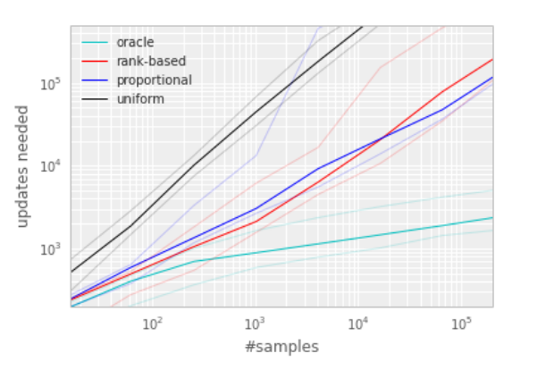
They achieved similar results for the Atari games. The greedy priorization techniques are rather easy to implement. That is the reason why I concentrate on the rank-based approach, guaranteeing better computation time with no significant loss in effectiveness to the proportional approach.
To draw a transition from a rank based distribution I constructed an example with sampling complexity $\mathcal{O}(1)$ avoiding calculating the cumulative sum of the priorities while sampling.
Concrete example - Geometric Series
For that we want to define a convex cumulative distribution function (CDF) $\Phi$ with $\Phi(0)=1$ and $\Phi(N)=0$.
My obvious choice was considering the geometric series, because of the explicit nature of calculating cumulative sums. On top we get another hyperparameter q taking the distribution:
$P(i)=1-\frac{q^{i}}{\sum_{j=1}^{N}q^{j}}$ with $0<<q<1$.
Remember the common procedure of drawing a random variable of a given distribution:
cum=0, rand=uniform
for m in memory:
    cum+=m.p
    if rand > cum:
        return m
That results in expense of $O(N)$ depending on memory size. Not to mention the cost it needs to calculate the fractions for $p_{i}$.
For the specific rank based distribution I suggested earlier I want to introduce a sampling method with constant time $O(1)$.
Define $S(n):=\sum_{i=1}^{N}q^i=\frac{1-q^{n+1}}{1-q}$
The Algorithm above formulates the recursive search after $\text{max}\begin{Bmatrix}n \in \mathbb{N} \mid \sum_{i=1}^{n}P(i) \leq \text{rand}\end{Bmatrix}$. This can be equally converted to the problem: $d(m)=\text{max}\begin{Bmatrix} n \in \mathbb{N} \mid S(n) \leq \text{rand} \cdot S(N)\end{Bmatrix} = \text{max}\begin{Bmatrix} n \in \mathbb{N} \mid S(n) \leq m \end{Bmatrix}$ where $m:=\text{rand} \cdot S(N)$ and $\text{rand}$ uniform in $[0,1]$
So let’s first transform the equation and then complete with floor function due to facing natural numbers for a real function.
$S(n) \leq m \Leftrightarrow \frac{1-q^{n+1}}{1-q} \leq \text{rand}\cdot\frac{1-q^{N+1}}{1-q} \Leftrightarrow \frac{1-q^{n+1}}{1-q^{N+1}} \leq \text{rand}$
Define $C:=\frac{1}{1-q^{N+1}}$. With that we get:
$C \cdot (1-q^{n+1}) \leq \text{rand} \Leftrightarrow 1-\frac{\text{rand}}{C} \leq q^{n+1}$
So applying logarithm we reveal $n \in \mathbb{N}$
$\log(1-\frac{\text{rand}}{C}) \leq (n+1) \cdot \log{q} \Leftrightarrow n \geq \log_{q}(1-\frac{\text{rand}}{C})-1$
With that we figured out that
$n = \lfloor \log_{q}(1-\frac{\text{rand}}{C})-1 \rfloor$
With that in mind out CDF looks like:
$\Phi(x)=\log_{q}(q^{N+1} + x \cdot (1 - q^N+1) )-1 \rfloor$
- Attention ceil instead of floor.
- Check Equations
- Explain Computation exeeds when percolating
- Heapify
- Manual for Heap Class